Introduction
Introduction.RmdThis short demonstration introduces some elementary capabilities of
the R package opendiscouRse.
Database setup
For the integrated Open Discourse database setup to work, you must set up database the database locally, e.g. by using Docker, as described here.
After configuring the database setup, we can obtain individual data
tables from the R6 class. In the following, we select the
politicians table.
od_obj <- OData$new()
politicians <- od_obj$get_table_data("politicians")$data
Usage of functions
count functions
count_data()
For simple data aggregations, we can use count_data() to
descriptively analyze the database. As we can see, the majority of
distinct politicians holding speeches in the Bundestag are men.
politicians |>
  count_data(grouping_vars = "gender")
#> # A tibble: 3 × 2
#> # Groups:   gender [3]
#>   gender       n
#>   <chr>    <int>
#> 1 männlich  3391
#> 2 weiblich   975
#> 3 NA          20
get functions
get_age()
Let’s move to generating new columns!
With the get_age() function, we can easily calculate the
age of politicians.
politicians |>
  dplyr::mutate(
    age = ifelse(
      is.na(death_date),
      # Alive politicians
      get_age(birth_date, round_val = 0),
      # Dead politicians
      get_age_hist(death_date, birth_date, round_val = 0)
    )
  ) |>
  dplyr::select(first_name, last_name, age) |>
  dplyr::slice(1:10)
#> # A tibble: 10 × 3
#>    first_name last_name   age
#>    <chr>      <chr>     <dbl>
#>  1 Manfred    Abelein      77
#>  2 Ernst      Achenbach    83
#>  3 Annemarie  Ackermann    81
#>  4 Else       Ackermann    86
#>  5 Ulrich     Adam         73
#>  6 Rudolf     Adams        94
#>  7 Raban      Adelmann     79
#>  8 Konrad     Adenauer     91
#>  9 Brigitte   Adler        60
#> 10 Eduard     Adorno       80
For substantive analyses, the type of profession is also interesting.
get_profession_groups() takes a data.frame
with information regarding the professional occupation, indicated in the
politicians data table, and returns a
data.frame with dummy variables indicating the profession
per group (we defined 7 profession categories).
get_profession_groups(politicians, "profession") |>
  dplyr::select(first_name, last_name, dplyr::starts_with("group_")) |>
  dplyr::slice(1:10)
#> # A tibble: 10 × 9
#>    first_name last_name group_recht group_wirtschaft group_naturwissenschaft
#>    <chr>      <chr>           <dbl>            <dbl>                   <dbl>
#>  1 Manfred    Abelein             1                1                       0
#>  2 Ernst      Achenbach           1                0                       0
#>  3 Annemarie  Ackermann           0                0                       0
#>  4 Else       Ackermann           0                0                       0
#>  5 Ulrich     Adam                0                0                       0
#>  6 Rudolf     Adams               0                0                       0
#>  7 Raban      Adelmann            0                0                       0
#>  8 Konrad     Adenauer            0                0                       0
#>  9 Brigitte   Adler               0                0                       0
#> 10 Eduard     Adorno              0                0                       0
#> # ℹ 4 more variables: group_gesellschaftswissenschaft <dbl>, group_agrar <dbl>,
#> #   group_journalismus <dbl>, group_handwerk <dbl>
When investigating the background of politicians, the affiliated
state (Bundesland) is politically of interest. State
affiliations get be obtained with get_state().
get_state(
  as.numeric(politicians$id),
  electoral_term = c(12, 17)
) |>
  table()
#>
#>      Baden-Württemberg                 Bayern                 Berlin
#>                     79                     99                     29
#>            Brandenburg                 Bremen                Hamburg
#>                     19                      5                     16
#>                 Hessen Mecklenburg-Vorpommern          Niedersachsen
#>                     45                     16                     62
#>    Nordrhein-Westfalen        Rheinland-Pfalz               Saarland
#>                    142                     36                     10
#>                Sachsen         Sachsen-Anhalt     Schleswig-Holstein
#>                     35                     20                     26
#>              Thüringen
#>                     22
For data visualization purposes (in party research), it is often
desired or at least advised to use colors that match parties (or
factions). get_faction_color() takes care fo that and
yields hex color codes that can be used to visualize parties
accordingly.
For that, we need to get a distinctive indication of political groups
acting in the Bundestag. Let’s load the factions table.
od_obj <- OData$new()
factions <- od_obj$get_table_data("factions")$data
get_faction_color(factions$abbreviation, id_type = "faction_name")
#>         <NA>          AfD          BHE           BP        Grüne      CDU/CSU
#>           NA    "#009EE0"    "#C3C318"    "#386ABC"    "#64A12D"    "#000000"
#>           DA   DIE LINKE.           DP       DP/DBP       DP/FVP          DPB
#>    "#000000"    "#BE3075"    "#63B8FF"    "#63B8FF"    "#63B8FF"           NA
#>          DRP       DRP/NR          FDP           FU          FVP Fraktionslos
#>    "#8b4726"    "#8b4726"    "#FFEE00"           NA    "#FFEE00"           NA
#>       GB/BHE         Gast           KO          KPD           NR          PDS
#>    "#C3C318"           NA           NA    "#8B0000"    "#8b4726"    "#BE3075"
#>          SPD          SSW          WAV            Z
#>    "#EB001F"    "#003C8F"    "#FFEC8B"    "#0000CD"
plot functions
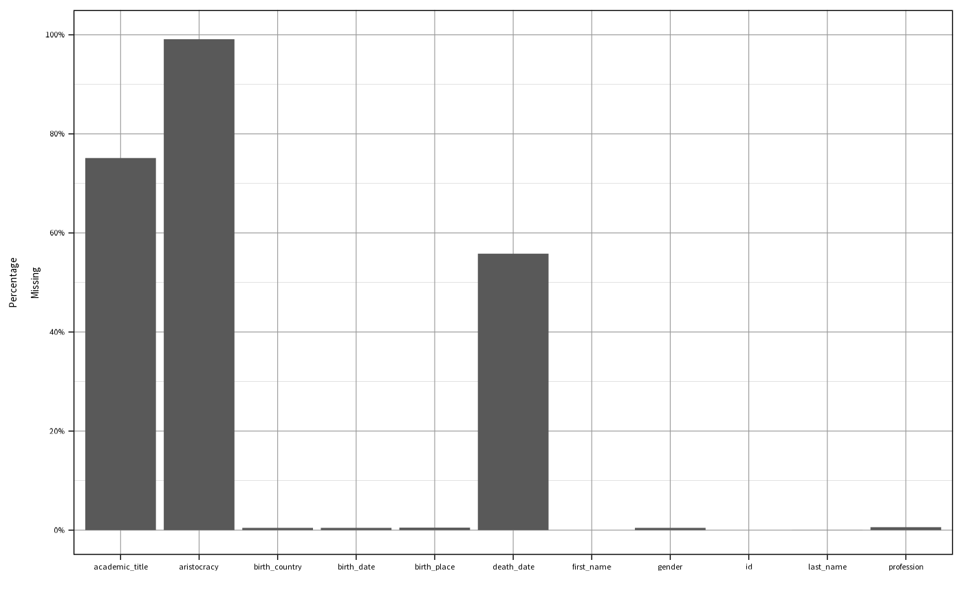
plot_cov()
The package comes with several plotting functions. For descriptive
purposes, we might be interested in the coverage of the data table.
plot_cov() visualizes NAs for the whole table.
Of course, there is a ggplot2 Open
Discourse theme.
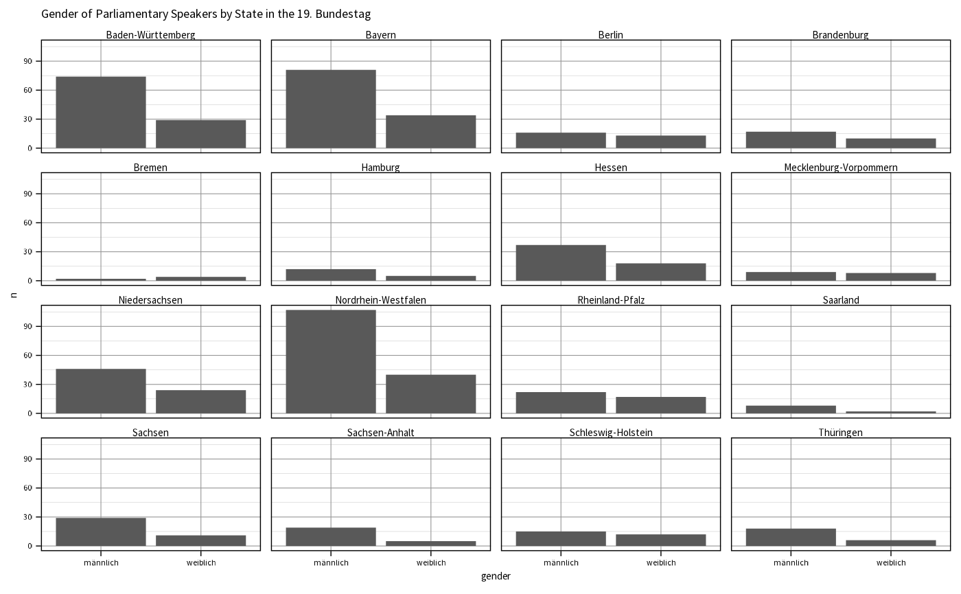
plot_count()
As shown above, count_data() computes counts per
grouping variables. plot_count() builds on that and is able
to visualize this type of counted data specifically. If we also
incorporate the Bundesland (state) affiliation through
get_state(), we can show how the distribution of gender
across states looks like.
politicians |>
  dplyr::mutate(state = get_state(id, electoral_term = 19)) |>
  dplyr::filter(!is.na(state)) |>
  count_data(grouping_vars = c("state", "gender")) |>
  plot_count(x_var = "gender", facet_var = "state") +
  theme_od() +
  ggplot2::ggtitle("Gender of Parliamentary Speakers by State in the 19. Bundestag")